How does an LLM work?

A typical autoregressive LLM reads text as tokens, processes them through a stack of Transformer layers built around the attention mechanism, and generates output one token at a time. This page walks through that pipeline: how text becomes tokens, what the model architecture looks like inside, and how inference proceeds through prefill and decode phases.

What are tokens and tokenization?

A token is the smallest unit of language that LLMs use to process text. It can be a word, subword, or even a character, depending on the tokenizer. Each LLM has its own tokenizer, with different tokenization algorithms.

Before text can be processed by the model, it must first go through tokenization. Tokenization is the process of splitting input text, such as a sentence or paragraph, into tokens.

Each LLM has a vocabulary: a fixed set of tokens the model can represent. Each token in the vocabulary maps to a token ID. During tokenization, tokens are converted into token IDs before being passed into the model during inference.

Here is a tokenization example for the sentence The quick brown fox jumps over the lazy dog. using GPT-5's tokenizer:

Tokens: "The", " quick", " brown", " fox", " jumps", " over", " the", " lazy", " dog", "."

Token IDs: [976, 4853, 19705, 68347, 65613, 1072, 290, 29082, 6446, 13]

For output, LLMs generate new tokens autoregressively. Starting with an initial sequence of tokens, the model predicts the next token based on everything it has seen so far. This repeats until a stopping criterion is met.

What's inside an LLM?

Most modern LLMs are decoder-only Transformer models. At a high level, the architecture has three major components:

1. Input representation: Token IDs are converted into numerical vectors (embeddings). The model also incorporates positional information so it can distinguish token order. For example, Rotary Positional Embeddings (RoPE) encode position within the attention computation.
2. A stack of Transformer layers: The embeddings pass through many Transformer layers. A typical layer combines a self-attention mechanism, which mixes information across tokens, with a feed-forward network, which transforms each token independently.
3. Output head: The final hidden state is projected into logits, one raw score for every token in the vocabulary. These logits are what the model samples from to pick the next token.

Many inference optimizations target either attention computation or the KV cache that attention uses during generation.

The attention mechanism

Attention lets the model assign different levels of importance to different tokens, so it can capture relationships across the sequence.

To do this, each attention layer learns three weight matrices: $W_Q$ (query weight), $W_K$ (key weight), and $W_V$ (value weight). These matrices are shared across all token positions and transform the hidden representation of each token into three vectors:

• Query (Q): A vector that represents a type of information the token wants to collect from the other tokens it can attend to.
• Key (K): A vector that represents the type of information the token offers. If the key vector is positively aligned with another token’s query vector, that other token will "attend to" this token (to a degree specified by an attention score, calculated based on how well the query and key vectors align).
• Value (V): A vector that represents the actual information the token offers to other tokens. If another token attends to this token, it will embed a proportion of this value into its token embedding (as determined by the attention score).

These three vectors allow the attention mechanism to determine how much each token attends to every other token, and what it takes away when it does. The model compares the query vector of the current token with the key vectors of all tokens it is allowed to attend to using a scaled dot product ($\frac{QK^\top}{\sqrt{d_k}}$). The resulting scores indicate how relevant each token is to the current one. Values play no role in this scoring step.

The scores are then normalized with a softmax function so they become attention weights that sum to 1. These weights determine how much each value vector contributes to the current token. Each value vector is multiplied by its attention weight, and the weighted values are summed together to produce the attention output for the current token, which updates its representation. In this way, each token incorporates information from other tokens according to how much attention it gives them.

In decoder-only LLMs, a causal mask limits each token to attending only to the current and earlier positions. This is how "bank" ends up meaning something different in "river bank" and "bank account": the representation of the token is updated based on the tokens it attends to.

The keys and values computed here are also what the model stores in the KV cache, which you'll see in the prefill and decode phases below.

For more information, see the Attention Is All You Need paper.

The attention mask

Self-attention can naturally look at every token in the sequence at once, but that's not always desirable. An attention mask controls which tokens each token is allowed to attend to.

For standard autoregressive generation, decoder-only LLMs apply a causal mask (also called a look-ahead mask). The mask is part of the architecture rather than an optional setting: an autoregressive model predicts the next token from the tokens before it, so a token must never see tokens that come after it. The causal mask enforces this by setting attention scores for future positions to negative infinity before softmax, so their weights become zero and no information flows from later positions to earlier ones.

The causal mask matters whenever many tokens are processed in parallel, such as during training and the prefill phase of inference. Without it, earlier tokens would attend to later ones, producing representations inconsistent with how the model generates text. During ordinary single-token decode, the model generates one token at a time and only past tokens exist in the KV cache, so there are no future positions left to mask.

Attention masks are also used to hide padding tokens, which are filler tokens added to align sequences of different lengths in a batch and carry no meaning of their own.

The two phases of LLM inference

For decoder-only Transformer models like GPT-4, the entire inference process breaks down into two phases: prefill and decode.

Prefill

When a user sends a query, the LLM's tokenizer converts the prompt into a sequence of tokens. The prefill phase begins after tokenization:

1. These tokens (or token IDs) are embedded as numerical vectors that the LLM can understand.
2. The vectors pass through multiple transformer layers, each containing a self-attention mechanism. Here, query (Q), key (K), and value (V) vectors are computed for each token. These vectors determine how tokens attend to each other (subject to the causal mask), capturing contextual meaning.
3. As the model processes the prompt, it builds a KV cache to store the key and value vectors for every token at every layer. It acts as an internal memory for faster lookups during decoding.

During the prefill stage, the entire prompt (namely, the whole sequence of input tokens) is already available before the LLM starts any actual computation. This means the LLM can process all tokens simultaneously through highly parallelized matrix operations, particularly in the attention computations.

As a result, the prefill stage is compute-bound and often saturates GPU utilization. The actual utilization depends on factors like sequence length, batch size, and hardware specifications.

A key metric to monitor for prefill is the Time to First Token (TTFT), which measures the latency from prompt submission to first token generation. More details will be covered in the inference optimization chapter.

Decode

After prefill, the LLM enters the decode stage where it generates new tokens sequentially, one at a time.

For each new token, the model samples from a probability distribution generated based on the prompt and all previously generated tokens. This process is autoregressive, meaning tokens T₀ through Tₙ₋₁ are used to generate token Tₙ, then T₀ through Tₙ to generate Tₙ₊₁, and so on.

The model can only predict tokens from its own vocabulary during decoding. A larger vocabulary can represent more text patterns directly, but it also makes the final prediction layer larger because the model scores every possible next token.

Use the stepper below to see the autoregressive loop in slow motion. Each click predicts one new token from the full sequence built so far.

Token-by-Token Decode Loop

Step through the decode loop. Each step picks one token from a distribution and appends it to the sequence.

Step 1 / 8

Sequence

T0Modular

T1is

T2a

T3unified

T4inference

T5?

Existing · 5Generated · 0Next

Next-token distribution

platform64%

stack18%

engine11%

service7%

KV cache

Reuses 5 cached K/V pairs; computes 1 new one this step.

Each newly generated token is appended to the growing sequence. This autoregressive loop continues until:

• A maximum token limit is reached,
• A stop word is generated,
• Or a special end-of-sequence token (e.g., <end>) appears.

Finally, the sequence of generated tokens is decoded back into human-readable text.

Compared with prefill, decode is more memory-bound because it requires the model weights and the growing KV cache to be frequently read from memory. KV caching stores these key and value matrices in memory so that, during subsequent token generation, the LLM only needs to compute the keys and values for the new tokens rather than recomputing everything from scratch.

This KV caching mechanism significantly speeds up inference by avoiding redundant computation. However, it comes at the cost of increased memory consumption, since the cache grows with the length of the generated sequence. KV cache memory can become a serving bottleneck even when the model weights already fit on the GPU. Some inference systems reduce this pressure by compressing or quantizing the KV cache, while others move inactive cache blocks to cheaper memory through KV cache offloading.

A key metric to monitor for decode is Inter-Token Latency (ITL), the time between the generation of consecutive tokens in a sequence.

Latency Timeline Visualizer

Press play to watch each decode step emit a token through detokenization. Pick a metric to see which stages it spans.

6 output tokens

Time to first token207 ms

Prompt submitted → first token shown

Tokenize + Prefill + Decode + Detok = 3 + 180 + 22 + 2

TTFT

0 ms · 0/6 tokensoutput appears here…

Tokenization Prefill Decode Detokenization

Assume Tokenization = 3 ms, Prefill = 180 ms, Decode = 22 ms, Detokenization = 2 ms, with ITL constant across decode steps. Real values vary with model, hardware, and sequence length.

Collocating prefill and decode

Traditional LLM serving systems typically run both the prefill and decode phases on the same hardware. However, this setup introduces several challenges.

One major issue is the interference between the prefill and decode phases, as they cannot run fully in parallel. In production, multiple requests can arrive at once, each with its own prefill and decode stages that overlap across different requests. However, only one phase can run at a time. When the GPU is occupied with compute-heavy prefill tasks, decode tasks must wait, increasing token latency, and vice versa. This makes it difficult to schedule resources for both phases.

The open-source community is actively working on different strategies to separate prefill and decode. For more information, see prefill-decode disaggregation.

What is a context window and how does it work in LLM inference?

The context window is the number of tokens an LLM can process in a single inference pass. It includes the entire conversation history that must be resent each turn to maintain coherence.

Context Window Simulator

Every turn, the full conversation is re-sent to the model. Watch the window fill up.

Model context size

Input to the model

All prior messages are re-sent every round.

Click + Add turn to start the conversation.

Token usage

0 / 32,000

0%of context used

Pick a model size, then add turns to see the input grow.

Technically, LLMs don’t have real memory. To keep context, every new request must resend all previous messages so the model can “see” the full conversation again (it happens under the hood and users don’t see it). In other words, continuity is maintained by reconstructing the context through the input prompt each time.

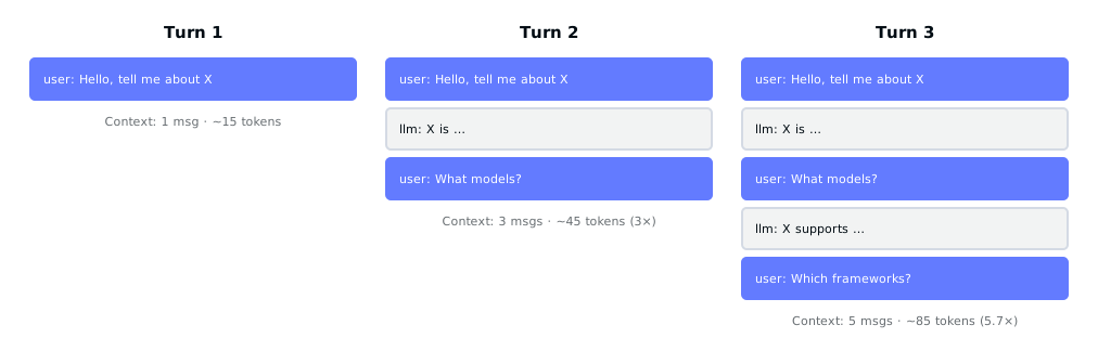
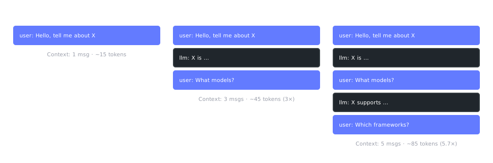
This running text history is called the context window, which has a maximum length (e.g., 8K, 32K, or 128K tokens).

As mentioned above, LLMs use the KV cache from previous tokens to avoid fully reprocessing everything in the decode phase, which helps with latency. When reusing the KV cache across multiple requests, it is more accurate to call this technique prefix caching.

Diffusion LLMs (dLLMs)

The autoregressive pattern of LLMs has a natural bottleneck: slow and computationally expensive.

Diffusion LLMs (dLLMs) flip that logic. They output the entire response in parallel through a denoising process inspired by image generation models like Stable Diffusion.

Here’s the basic idea:

1. The model starts with a cloud of noise, representing a rough sketch of possible outputs.
2. Through several denoising steps, it gradually refines that noise into coherent text.
3. The final answer emerges all at once, like an image coming into focus.

This parallel process removes the token-by-token bottleneck. It also allows dLLMs to iterate and self-correct during generation, which makes them particularly strong at tasks like editing, mathematical reasoning, and code completion.

Early examples of dLLMs include:

• Mercury by Inception AI: reportedly delivers inference up to 10× faster and more efficient than traditional LLMs.
• Gemini Diffusion by Google DeepMind: an early exploration of applying diffusion to text generation. It is available as an experimental demo to help develop and refine future models.

For now, autoregressive LLMs remain the mainstream architecture. However, dLLMs represent one of the most promising directions to power the next generation of inference systems. If you’re working with autoregressive LLMs today, it’s worth keeping an eye on dLLMs.

FAQs

Are all LLMs decoder-only Transformer models?

No. LLMs can be built using different Transformer architectures, including encoder-only, encoder-decoder, and decoder-only models.

However, when people talk about LLMs today, they are usually referring to decoder-only Transformer models. They dominate modern generative AI applications such as chatbots and coding assistants. Most inference techniques discussed today, including KV caching, continuous batching, speculative decoding, and prefill-decode disaggregation, are designed around this architecture.

Architecture	Examples	Prefill and decode phases	Note
Encoder-only	BERT, RoBERTa	No. The input is processed in a single forward pass with no autoregressive generation.	Mostly used for classification, embeddings, and search
Encoder-decoder	T5, FLAN-T5, BART	Partially. The encoder processes the input once, while the decoder generates tokens autoregressively.	Less common for frontier LLMs
Decoder-only	GPT, Llama, Qwen, DeepSeek, Claude	Yes. Inference consists of a prefill phase followed by a token-by-token decode phase.	The dominant architecture for modern LLMs

Unless stated otherwise, "LLM" in this handbook refers to decoder-only Transformer models.

What is KV cache?

The KV cache is the memory an LLM uses to store the key (K) and value (V) vectors it has already computed, so it doesn't have to compute them again.

Attention works by having each token attend to every token before it. Without a cache, generating token 1,000 would mean recomputing the keys and values for the 999 tokens that came first, then repeating that work for token 1,001. Because those vectors depend only on the tokens themselves and not on what comes after, they never change once computed. Caching them turns each decode step into computing K and V for a single new token and reading the rest back from memory. This is how the KV cache mecahnism helps speed up inference.

As the sequence length grows during inference, the KV cache becomes the dominant factor in memory usage. For Llama 3 8B in FP16, for example, a single 8K-token sequence holds about 1 GB of KV cache (learn more about the calculation). The weights take roughly 16 GB. On an 80 GB GPU, this leaves at most around 64 GB for the KV cache and other runtime data, giving a theoretical upper bound of roughly 60 such sequences. This is why the KV cache, not the model weights, is usually what limits how many users a server can handle.

The KV cache is the thing several optimization techniques in this handbook are built around:

• PagedAttention stores the cache in fixed-size blocks to avoid fragmentation and over-reservation
• Prefix caching reuses the cache for a shared prompt prefix across requests
• KV cache offloading moves inactive blocks to CPU memory or disk, and includes a calculator for the example above
• Prefill-decode disaggregation splits the two phases across workers and transfers the cache between them

How are tokens selected via sampling?

At each decode step, the model does not directly output a word. Instead, it produces a probability distribution over all possible tokens.

Sampling is the process of selecting the next token from this distribution.

Before sampling, temperature is applied to the logits (the raw pre-softmax scores). It rescales them, which changes the shape of the distribution before probabilities are computed.

• Lower temperature: the distribution becomes more peaked (a few tokens dominate)
• Higher temperature: the distribution becomes flatter (probability spreads across more tokens)

After applying temperature and converting logits into probabilities, a sampling strategy determines which token gets picked. Common ones include greedy decoding, top-k, and top-p.

Learn more about LLM inference parameters.

What happens step by step during LLM inference?

At a high level, LLM inference follows a simple loop:

1. The input text is converted into tokens
2. Tokens are processed in the prefill phase to build context and KV cache
3. The model enters the decode phase. At each step:
   • The model produces a probability distribution
   • A sampling strategy selects the next token
4. The process repeats until a stopping condition is met
5. Tokens are converted back into readable text

Even though the output feels instant, this process runs one token at a time during decoding.

Why is LLM inference slow?

LLM inference can be slow for two main reasons:

• Sequential decoding: tokens are generated one by one, which limits parallelism
• Memory bottlenecks: during decoding, the model repeatedly reads from KV cache in GPU memory

Other factors also affect latency:

• Model size (more parameters mean more computation)
• Input length (longer prompts increase prefill time)
• Hardware (GPU type and memory bandwidth)

This is why inference optimization is a major focus in production systems.

Additional resources

• DistServe: Disaggregating Prefill and Decoding for Goodput-optimized Large Language Model Serving
• Large Language Diffusion Models